1D Linear Advection

The Semi-Lagrangian Method

We have observed how the CFL number can affect the numerical solution of the 1D linear advection wave equation.

Hitherto, our computations have been on a fixed set of points giving the Eulerian description of the advection problem. The alternative is to "go with the flow", i.e. let the initial discrete grid evolve over time. This Lagrangian description results in the initial grid becoming distorted as the particles are advected from their initial state. The compromise is the "Semi-Lagrangian" approach considered here. Semi-Lagrangian methods have proved to be popular especially in the highly demanding discipline of numerical weather prediction.

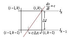
We note that along any characteristic line $$\frac{dx}{dt}=c$$ and $$\frac{D\phi}{Dt}=0$$ i.e. $$\phi$$ is conserved along characteristic lines. Thus we can draw the characteristic line from grid point $$(x_i,t_k)$$ to $$(x_i-c\Delta x,t_{k-1})$$. First $$x_{i-1}$$ is determined as shown in the figure to the right.

Since $$\phi(x_i,t_{k-1}), i=0,...,N_x$$ is known, we use interpolation to compute $$\phi(x_i-c\Delta x,t_{k-1})$$.

In simple cases linear interpolation can be used. In more complicated cases, a three-step procedure is used to calculate $$x_i-c\Delta t$$ and cubic interpolation ensures accurate solutions. Interpolation ensures that the CFL condition is satisfied.