Prev

Introduction

Next

We use a simple example of incompressible turbulent flow as a means of introducing engineering students to turbulent flow without recourse to a physical description of the different regimes of wall bounded turbulent flows or the rigor of asymptotics, both of which are necessary and appropriate in an advanced engineering course (see, for example, [9]). Here, we use an empirical polynomial approximation of fully developed streamwise velocity profile in a plane channel due to Pai [2]. This problem has been the focus of major experimental and computational analysis in the second half of the twentieth century and continues to reveal novel microscopic features thanks to increased supercomputing resources.

Visual examples of turbulent flow

Turbulent Flows - 1 / 11

Prev

Fully Developed Turbulent Flow

Next

Here, we briefly describe the equations of fully developed turbulent flow in a plane channel. Further details can be found in classical references (see, for example, [9]). The Reynolds hypothesis for turbulent flow assumes that the velocity \( \left( u, v, w \right) \) and pressure \( p \) are decomposed into a mean component and a fluctuating component, i.e.

\[ \left( u , v , w, p \right) = \left( \bar{u}, \bar{v}, \bar{w}, \bar{p} \right) + \left( u^\prime , v^\prime , w^\prime , p^\prime \right) \]

where the mean is usually taken over a finite time interval. Consequently, the nonlinear terms in the Navier-Stokes equations generate additional terms called the Reynolds stresses.

In the case of fully developed incompressible two-dimensional flow in a plane channel the Reynolds averaged Navier-Stokes equations reduce to:

\begin{align} \frac{\partial \bar{p}}{\partial x} & = \frac{d}{dy}\left(\mu\frac{d\bar{u}}{dy} - \rho \overline{u^\prime v^\prime}\right) \tag{1A} \\ \frac{\partial \bar{p}}{\partial y} & = -\frac{d}{dy}\left(\rho\overline{v^n}\right) \tag{1B} \end{align}

where \( -\rho\overline{u^\prime v^\prime} \) and \( -\rho\overline{v^n} \) are the Reynolds stresses, or second-order moment tensors as they are sometimes called. Unfortunately, to close the problem the transport equations for the second-order moment tensors generate third-order moment tensors and so on. This problem of closure has been the bane of turbulence modeling for over the past hundred years.

Turbulent Flows - 2 / 11

Prev

Approximating Closure

Next

A starting point is the Boussinesq approximation [9]

\[ -\rho\overline{u^\prime v^\prime} = \mu_\tau \frac{d\bar{u}}{dy} \tag{2} \]

which introduces the turbulent viscosity \( \mu_\tau \) int erms of known quantities such as \( \bar{u} \) or turbulent kinetic energy \( k = \left( \overline{u^n} + \overline{v^n} + \overline{w^n}\right) / 2 \) depending on the choice of the turbulence model (e.g. the Prandtl mixing length hypothesis or the \( k - \varepsilon \) turbulence model still used in major commercial computational fluid dynamics). The Boussinesq approximation assumes that the flow is isotropic when in wall bounded flows the flow is in fact anisotropic.

Integrating equation (1) with respect to why yields

\[ p + \rho\overline{v^n} = P_w\left( x\right) \tag{3} \]

where \( P_w\left( x\right) \) is the pressure on either wall of the channel. Let us define the total shear stress as \( \tau := \mu\frac{du}{dy} - \rho\overline{u^\prime v^\prime} \). The integrating equation (2) yields

\[ \tau = -\left( H - y\right)\frac{dP_w}{dx} \tag{4} \]

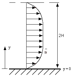
where \( H \) is the half-width of the channel. The wall shear stress at \( y = 0 \) given by \( \tau_w \) is \( -H\frac{dP_w}{dx} \). It is useful to define a friction velocity \( u_\tau^2 = \frac{\tau_w}{\rho} \). Then if

\[ r = \frac{\overline{u^\prime v^\prime}}{u_\tau^2} , V = \frac{u}{u_\tau} , \eta = \frac{y}{H} , R_\tau = \frac{u_\tau H}{v} \]

equation (4) reduces to

\[ -r = \frac{1}{R_\tau} \frac{dV}{d\eta} - \left( 1 - \eta \right) \tag{5} \]

Turbulent Flows - 3 / 11

Prev

Empirical Approximation of Velocity

Next

To determine \( r \) we use an empirical polynomial approximation for the velocity \( V_e := \frac{\bar{u}}{u_m} \) (where \( u_m \) is the maximum velocity on the centerline) obtained by Pai [2]

\[ V_e = 1 - \left( \frac{n-s}{n-1}\right)\left( 1 - \eta\right)^2 - \left( \frac{s-1}{n-1}\right)\left( 1 - \eta\right)^{2n} \tag{6}\]

where \( s = \frac{R_\tau^2}{2R_m} \) and \( n \) is a positive integer. Note that the laminar case is recovered when \( s = 1 \), and turbulent flow exists when \( s > 1\).

By comparing equation (6) to Laufer's experimental data [13], Pai observed that \( n = \gamma s \) where \( \gamma = 1.4 \). We have previously shown that \( \gamma \) is sensitive to \( R_m \) [3]. Pai plotted \( V_e \) and \( -r \) for \( R_m = 12300 \). We emphasize that equation (6) is an approximation and not an exact solution of Reynolds averaged equations. In the following, we assume taht \( R_m = 12300 \). The corresponding value of \( R_\tau \) may be determined from the empirical formula of Hussain and Reynolds [1], \( R_\tau = 0.1079 R_m^{0.911} \) which gives in this case \( R_\tau = 574.02 \).

It is common to use two scales in analyzing wall bounded turbulent flows. One is the outer wall variable given by \( \eta \) and the other is the inner wall variable \( y^+ = \eta R_\tau \); likewise the outer velocity is \( \frac{U}{U_m} \) and inner wall velocity \( u^+ = \frac{u}{u_\tau} \). These scales may easily be inferred from physical arguments or matched asymptotic expressions [9].

Turbulent Flows - 4 / 11